Tigre Municipality: Citizen Satisfaction Analytics

A project in two chapters

In 2023, I worked with the Environmental Secretary of Tigre’s Municipal Council to turn 7,824 citizen survey responses into interactive Power BI dashboards for the Mayor’s office. The report covered everything from demographic breakdowns to service-by-service satisfaction ratings across Tigre’s twelve localities.

When I came back to the project in 2025 to update my portfolio, I kept thinking about one persistent pain point from the original work: extracting keywords from open-text survey responses had been done manually by pollsters, resulting in thousands of inconsistent labels. It seemed like exactly the kind of problem worth revisiting properly.

So I rebuilt that piece from scratch — this time with a proper unsupervised NLP pipeline that discovers keyword categories purely from the text, with no human labels as input.

---

2023: The survey analytics project

Context

Tigre’s Environmental Secretary ran a citizen satisfaction survey between September 2021 and December 2022. The goal was to measure how residents felt about local government services, segment results by demographic and geography, and give decision-makers something actionable.

• 7,824 residents surveyed through in-person structured interviews
• Target population: all inhabitants aged 16+ across 12 localities
• Survey structure: 6 multiple choice questions, 14 Likert-scale ratings (1–7), and 2 open-text fields

The survey also included two open-text fields — one for complaints and suggestions, one for positive feedback — where respondents could mention specific municipal services in free-form language.

What I built

After cleaning the data and structuring it into a proper data model, I built six interconnected Power BI dashboards covering respondent profiles, local government image, service-level satisfaction, claims, commendations, and top neighborhood problems.

---

2025: Unsupervised NLP extension

The original keyword problem

The two open-text fields were the richest data in the survey. But when it came to extracting keywords — classifying each response under a service category like “Cleaning”, “Security”, or “Streets” — that work was done manually by the survey team. The result was thousands of inconsistent labels: typos, mixed granularity, missing values, and categories that overlapped.

In 2025 I decided to redo this properly, treating it as an unsupervised keyword extraction problem. The constraint I set myself: no human labels as input. Every category would be discovered purely from the text.

Approach: multi-method ensemble + semantic clustering

I combined four complementary extraction methods, each capturing a different signal from the text:

Method	What it captures
YAKE	Statistical patterns — position, frequency, co-occurrence. Fast, no model needed.
KeyBERT	Semantic similarity via multilingual BERT embeddings. Understands meaning across synonyms.
spaCy noun chunks	Syntactic structure via dependency parsing. Extracts root nouns from noun phrases.
TF-IDF	Corpus-level discrimination — what makes this response different from all others.

The four methods vote on each candidate keyword with weighted scores (YAKE 1.0, KeyBERT 0.8, noun chunks 0.7, TF-IDF 0.6). Keywords found by multiple methods accumulate higher confidence. For very short responses (under 15 characters), KeyBERT’s weight drops to 0.3 since it can’t build meaningful embeddings from minimal context.

After collecting raw keywords across all 7,824 responses, a semantic clustering step groups similar keywords into canonical categories. Each keyword is embedded using the same multilingual BERT model, then Agglomerative Clustering with cosine distance auto-discovers the natural groupings. The most frequent member of each cluster becomes its label — so “robo”, “cámara”, “seguridad” all collapse into a single Seguridad category.

Results

Comparing against the original human labels as a hidden test set at the end:

Metric	Complaints	Positives
Exact match	13.8%	39.8%
Fuzzy match	17.0%	42.6%
F1 Score	32.8%	52.2%

The lower scores for complaints are partly expected — human labels for complaints were more inconsistent to begin with, and the pipeline extracts the most salient keyword where humans sometimes assigned multiple overlapping categories. A side-by-side sample illustrates both where it works and where it misses:

Unsup: [Veredas          ]  Human: [Veredas          ]  ✓  "Arreglar la desnivelación de las veredas."
Unsup: [Calles           ]  Human: [Calles            ]  ✓  "Que arreglen las calles."
Unsup: [Camaras Seguridad]  Human: [Seguridad         ]     "Más seguridad, quiere que pongan más cámaras."
Unsup: [Veredas          ]  Human: [Residuos          ]     "No está pasando el barrendero."

The third example is technically accurate but too specific; the fourth extracts a surface noun (“veredas” = sidewalks) when the real topic is trash collection. Both are fixable with better post-processing — but for an approach that never saw a single label during training, it holds up reasonably well.

---

2023 — Technical implementation

Data exploration (Python / Pandas)

Before touching Power Query, I ran a Python EDA pass to understand the shape and quality of the data (explore_data.py). The key things it surfaced:

• 7,824 rows × ~60 columns after removing fully-blank rows
• Several columns with >30% null rates, mostly optional follow-up questions
• Rating columns had stray text values that needed coercion to numeric
• The open-text fields (15.RECLAMO PARA DERIVAR, 32.ASPECTO POSITIVO) had highly variable lengths — some single words, some multi-sentence paragraphs
• The manually-assigned keyword columns (Reclamos y sugerencias- Palabras, Positivo- palabras) were present but inconsistent

The EDA output includes charts for missing value distribution, demographic breakdowns, satisfaction rating means, and locality coverage.

Data cleaning (Power Query)

The raw Excel data, entered manually from physical forms, needed substantial cleaning before it could be modeled. Key transformations in Power Query (m-code-powerquery-cleaning.txt):

Structural cleanup

• Promoted headers and enforced explicit data types on all 60+ columns
• Removed fully-blank rows and columns with no analytical value (e.g. Column67, contact fields)
• Dropped binary flag columns used only for internal tracking

Text normalization

• Trimmed and lowercased the Positivo- palabras keyword column
• Replaced abbreviation variants ( led → removed, lomas de burro → lomadeburro) for consistent grouping
• Added a sequential index column for use as the relationship key to the Claims and Commendations lookup tables

Column renaming All raw Spanish column names were standardized to cleaner display labels (e.g. 15.RECLAMO PARA DERIVAR → Reclamos Texto Abierto, 32.ASPECTO POSITIVO → Valoración Positiva Texto Abierto).

Category regrouping in Power BI

The human-labeled keyword columns still had too much granularity after cleaning — dozens of specific variants where five or six canonical categories were sufficient for the dashboards. This final grouping was done directly in Power BI using group editing on the category columns, collapsing related terms into the service categories visible in the Claims and Commendations dashboards (Streets State, Cleaning, Security, Lightning, Sewers, Green Spaces, Sports & Culture, etc.).

Data model

The logical model follows a simple star schema with the survey as the central fact table and two derived dimension tables built from the keyword columns.

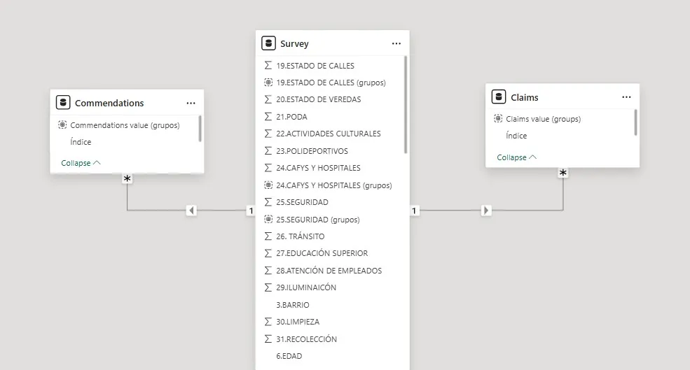
• Survey — fact table, one row per respondent, contains all Likert ratings, demographics, and open-text fields
• Claims — one row per keyword extracted from the complaints field, linked back to Survey via index
• Commendations — same structure for the positive feedback field
• Electores por Localidad — voter counts by neighborhood, used for population weighting
• Messures — calculated measures table (averages, percentages, counts for KPIs)

Relationships are many-to-one from Claims/Commendations to Survey, enabling cross-filtering between the open-text dashboards and all demographic slicers.

Power BI dashboards

Six report pages with consistent navigation, a shared slicer panel (Suburb, Gender, Age, Educational Level), and an “Erase all segmentations” reset button on each page. All charts cross-filter across pages when drilling into a specific demographic or locality.

---

2025 — NLP pipeline technical detail

Text cleaning (text_cleaning.py)

All open-text responses pass through a shared cleaning pipeline before any extraction method sees them:

1. Lowercase and strip punctuation (preserving accented Spanish characters)
2. Collapse whitespace
3. Lemmatize using spaCy’s es_core_news_md model
4. Remove Spanish stopwords plus a custom survey-specific list (SURVEY_STOPWORDS) of words that appear everywhere but carry no keyword meaning — “vecino”, “barrio”, “pide”, “arreglar”, and similar.

Multi-method extraction (unsupervised_extractor.py)

YAKE runs per-document with Spanish language settings, extracting up to 5 bigram candidates. Scores are inverted (lower YAKE score = higher importance) before entering the ensemble. Works well even on single-sentence responses.

KeyBERT uses paraphrase-multilingual-MiniLM-L12-v2 (~120MB, supports 50+ languages). It embeds the full document and each candidate phrase, then returns the 5 phrases with embeddings closest to the document vector. Maximal Marginal Relevance (diversity=0.5) prevents redundant candidates. Weight drops from 0.8 to 0.3 for texts under 15 characters.

spaCy noun chunks extracts the root noun from each dependency-parsed noun phrase, lemmatizes it, and also sweeps for individual nouns and proper nouns not captured by chunks. All candidates receive a uniform score (1.0 for chunk roots, 0.8 for individual nouns) since spaCy doesn’t rank them.

TF-IDF is fit on the full corpus (TfidfVectorizer, max 500 features, bigrams, min_df=3, max_df=0.5). Per-document, it returns the top 5 terms by TF-IDF weight — what makes this specific response distinctive relative to all others.

The ensemble sums weighted scores across all four methods. Any keyword found by multiple methods accumulates higher total weight and rises to the top. The final output is the top 1–2 candidates per response.

Category discovery (category_discovery.py)

Raw keywords across the full corpus are aggregated and filtered to those appearing 3+ times (removes noise and one-off typos). The remaining vocabulary — typically 200–500 unique terms — is embedded with the same multilingual BERT model.

Agglomerative Clustering with metric="cosine", linkage="average", and distance_threshold=0.35 groups semantically similar keywords without requiring a pre-specified number of clusters. The most frequent keyword in each cluster becomes the canonical category label. This produces a lookup table mapping raw extracted terms to canonical categories, replacing the hand-crafted regex dictionary entirely.

Validation (validation.py)

Three levels of comparison against the original human labels (used only as a hidden test set at the end):

• Exact match — normalized string equality after removing accents
• Fuzzy match — fuzz.token_sort_ratio handles different keyword ordering (“Seguridad Limpieza” vs “Limpieza Seguridad”)
• Keyword-level precision / recall / F1 — treats each row’s keywords as a set; compares predicted set against the first two human-assigned keywords for a fair comparison (since the pipeline extracts max 2)

Coverage (the percentage of non-null input texts that receive at least one keyword) consistently exceeded 85% on both the complaints and positives columns.

What I would do differently

The ensemble approach worked, but it’s complex to maintain — four models with different output formats, normalization pipelines, and tunable weights. If I were starting fresh today, I’d replace most of this with a single LLM call using structured outputs. One well-prompted model handles extraction, normalization, and categorization in a single pass with better semantic consistency and far less code. The unsupervised clustering step would still be useful for discovering the category taxonomy before writing the prompt, but the per-document extraction step becomes much simpler.